Bayesian VAD: Fixing turn detection in production voice pipelines

When a voice AI agent cuts a customer off mid-sentence, the interaction feels dismissive and erodes the trust that enterprise deployments depend on.

Most voice AI agents run on a cascade pipeline: speech-to-text (STT), agent logic, then text-to-speech (TTS). Each stage inherits the errors of the last, which makes detecting when someone is done speaking and reliably converting it to text particularly consequential.

The problem is especially acute in customer support. Callers call in from noisy environments, switch between languages mid-conversation, and rarely speak in well-punctuated sentences. The pipeline has to handle all of it.

The typical speech-to-text path looks like this:

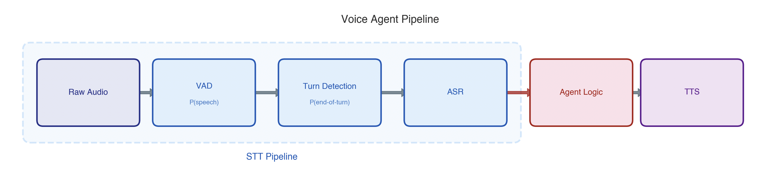
• Voice Activity Detection (VAD) estimates the probability of speech occurring in each audio frame.
• Turn detection estimates the probability of the user is actually done talking.
• Automatic Speech Recognition (ASR) transcribes the accumulated audio to text.

After analyzing production audio at scale, we found that premature turn endings (i.e., the agent jumping in before the user is done) account for the majority of VAD-based errors. We discovered two root causes: the underlying probabilities are poorly calibrated for real-world audio, and thresholding individual frames is simply the wrong tool for making turn decisions.

We developed novel statistical methods to solve each without retaining any models. The result was 42% fewer broken turns and a 20% reduction in transcription error.

Measuring STT

Before fixing anything, we needed to measure the right things. STT has two jobs: detect user turns and transcribe them. A user turn is a complete start-of-speech to end-of-thought segment spoken by the user. Each requires its own ground-truth and metrics.

Detection metrics

Three things matter for turn detection:

• Did we find the right boundaries (i.e., the start and end timestamps of the turn)?
• Did we accidentally split a single turn into multiple segments?
• How quickly did we commit to a decision?

Transcription metrics

The industry standard for transcription quality is Word Error Rate (WER), but standard practice has a blind spot. It feeds clean, ground-truth audio segments directly to ASR and reports WER on those. This hides detection errors entirely. If the system only captured half a turn, a perfect transcription still looks like 50% accuracy to the user.

To address that gap, we developed Pipeline WER, a conversation-level metric that includes fragmented and missed turns. It uses a simple sentinel decomposition approach that we prove is equivalent to the theoretically correct per-turn WER (see Appendix).

We determine the right sample size for these metrics by computing an incremental stability statistic over the data. (see Appendix).

Turn-taking problems

So where do the premature turn endings come from?

VAD models are extremely responsive and handle speech start just fine. The failures are entirely on the end-of-turn side and trace back to two structural issues.

Problem 1: Miscalibrated probabilities

Off-the-shelf VAD models are trained on clean speech corpora. Deploy them on real-world audio (e.g., noisy environments, accented speech, cross-talk) and the probabilities they output are wrong.

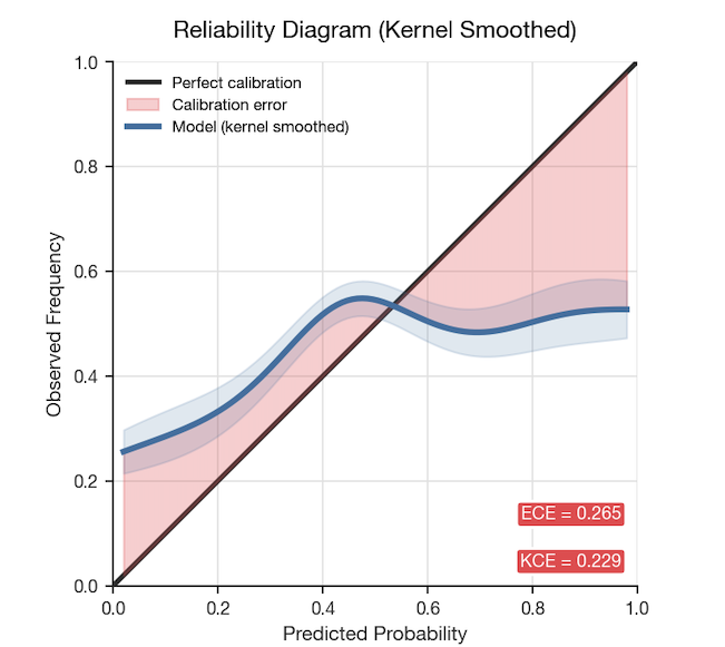
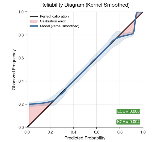
Fixing calibration: Isotonic regression

To remap model outputs to true probabilities, we applied isotonic regression — a technique that fits a monotone mapping from predicted to observed probabilities:

Optimized via the Pool Adjacent Violators Algorithm (PAVA), the results are striking:

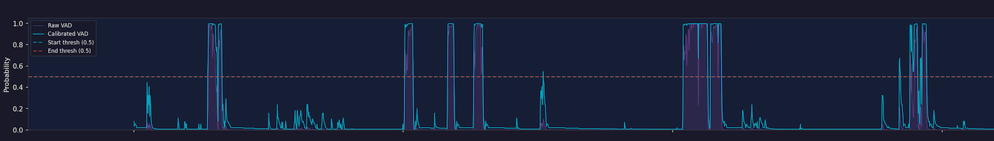
Plotting raw (purple) versus post-isotonic (cyan) probabilities on a sample conversation shows the difference clearly. Probabilities are now meaningful, but the sharp dips remain:

Calibration alone gains 1–2pp in turn boundary precision/recall since we can more easily find the optimal threshold, but the fundamental issue of reacting to individual frames is still unresolved. That’s the second structural issue.

Problem 2. Wrong decision framework

Even with well-calibrated probabilities, the standard approach to turn detection is fundamentally flawed.

The typical method relies on two heuristics: threshold a single VAD frame to detect silence, then wait a fixed timeout before committing to a turn end. The problem is that VAD outputs are inherently noisy: plosives, breaths, and natural inter-word pauses all produce momentary dips in the speech probability signal. Every dip is an opportunity for a false turn ending.

Per-frame thresholding is asking the wrong question. Instead of "is speech absent right now?", the right question is: "given everything observed so far, is there enough accumulated evidence that the speaker is actually done?"

Bayesian hazard statistic

To answer that question, we developed a new decision statistic that replaces both heuristics with a single learned statistic, cutting broken turns by 42%. The construction has two steps.

Step 1: Define “Evidence of silence”

Step 2: Define “evidence speaker is done”

Knowing how much silence has accumulated isn't enough on its own. We also need to find the rate at which turns actually end given a level of accumulated silence evidence. This is a hazard function:

The cumulative hazard over silence evidence gives the total evidence of a true turn end given silence evidence so far — the decision statistic we actually want to threshold on.

Effect on the signal

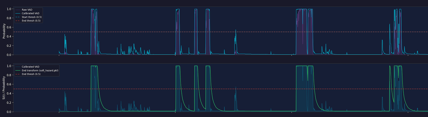
Plotting all three signals on the same conversation makes the improvement visible. The raw VAD probabilities (purple) are jagged and reactive. Post-isotonic regression (blue) is better calibrated but still noisy. The Bayesian hazard statistic (green) smooths out the within-speech dips and responds decisively to genuine silence:

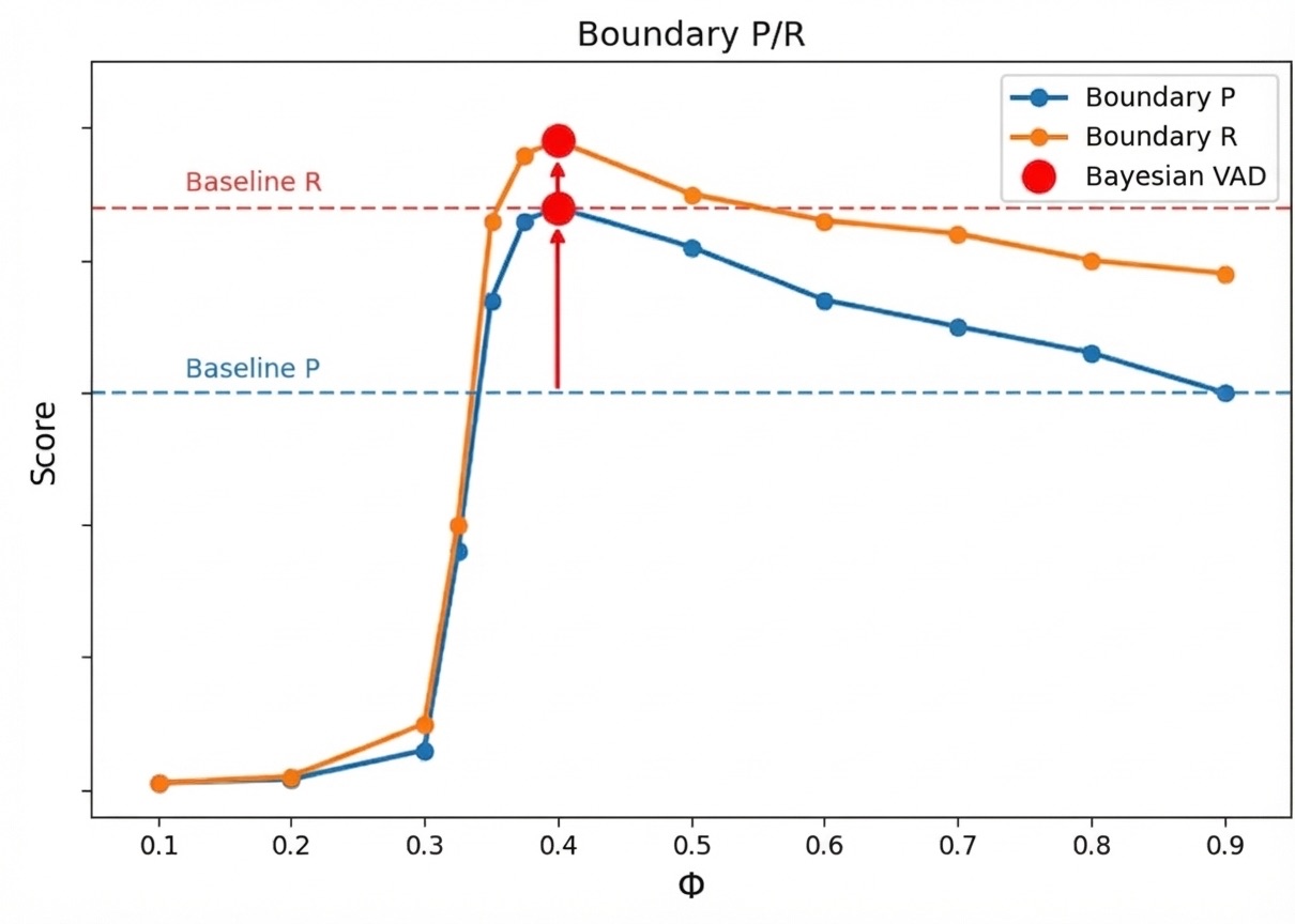
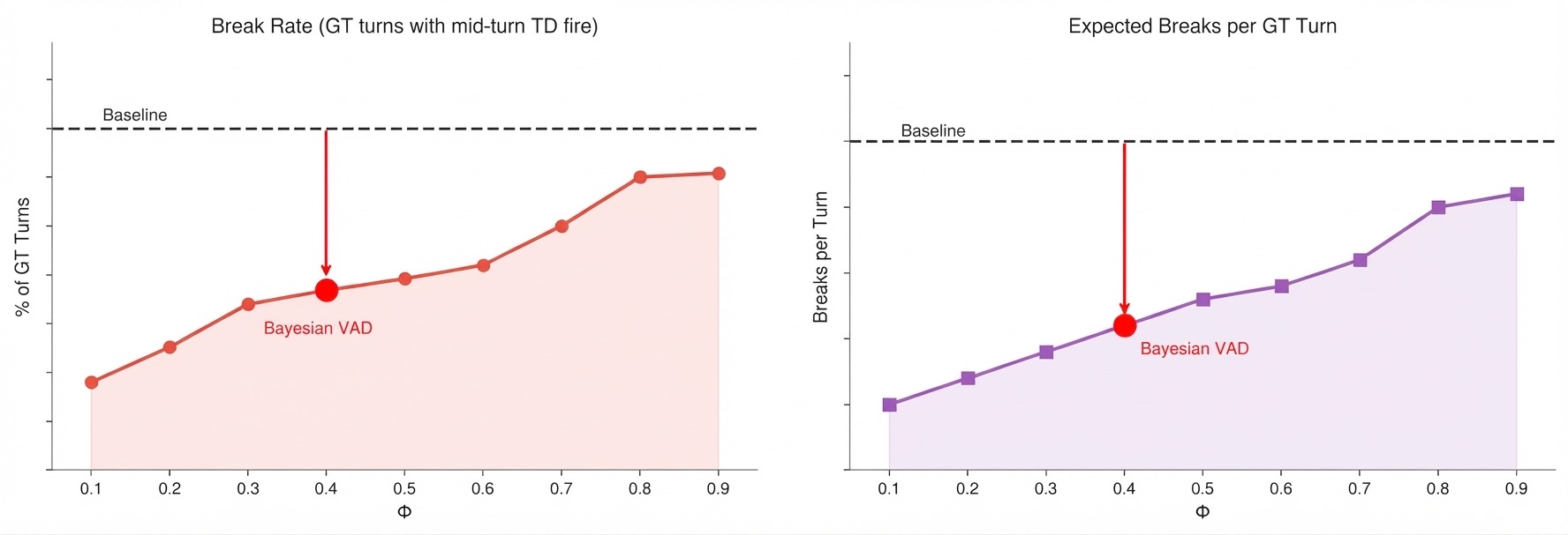
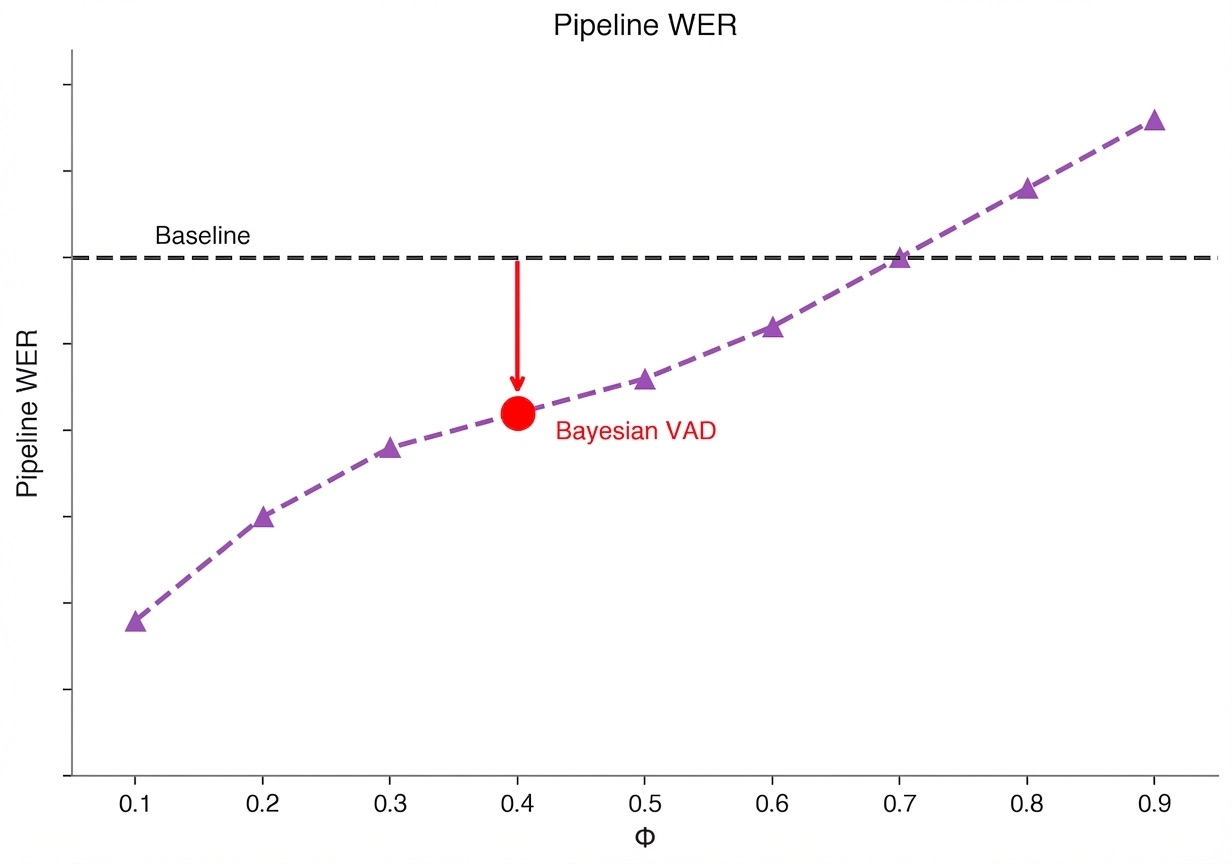
Results

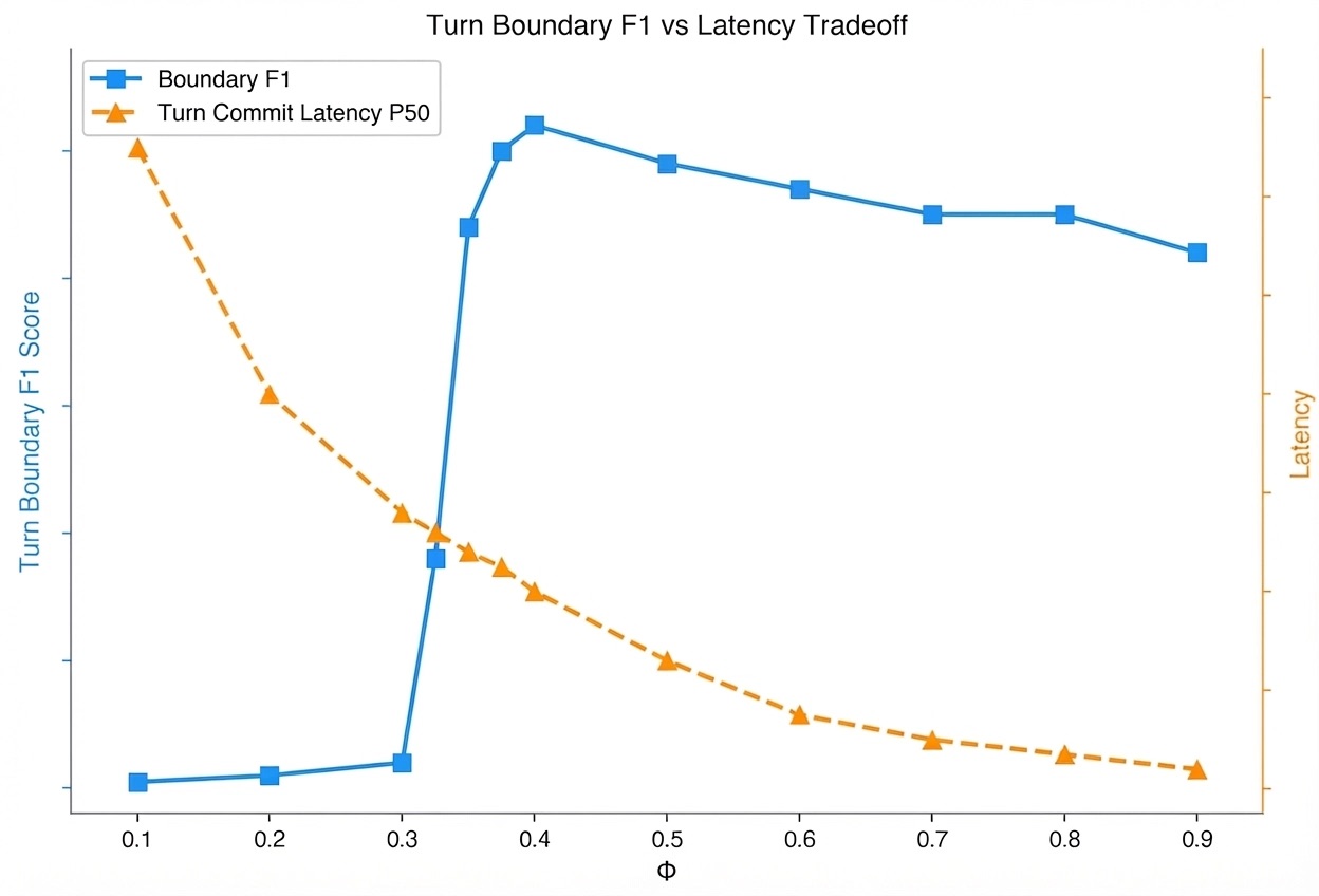
We found isotonic calibration and the hazard statistic improved every metric across the board. Because the hazard statistic is a proper evidence-accumulation framework, it also gives us a smooth, theoretically grounded tradeoff between decision latency and accuracy.

Turn detection accuracy

• 43% improvement in turn boundary precision
• 14% improvement in turn boundary recall

Turn breaks

• 42% reduction in broken turn rate
• 44% reduction in expected breaks per turn

Pipeline WER

• 20% reduction in pipeline WER

Latency–accuracy tradeoff

None of this required retraining a model or changing any architecture. The gains came entirely from fixing calibration and replacing a broken decision heuristic with one grounded in the right statistical framework.

The lesson generalizes. Before reaching for a better model, it's worth asking whether the framework around the model is sound.

Appendix

Pipeline WER

Proof

Metric Stability